Logistic Regression: Cost Function and Gradient Descent

The cost function:

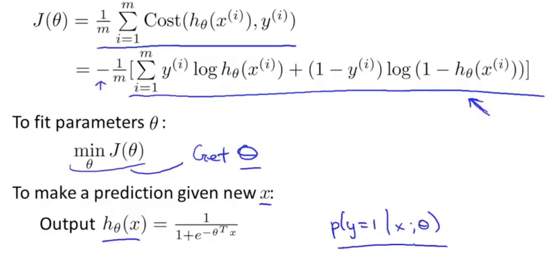
The cost function for Logistic regression is defined as follows:

$J(theta)$ is: \[(1/m) * ⅀cost( h(x(i), y) ) \] where the summation runs for all i.

Where Cost is defined as follows:

                                    $Cost(h(x), y) =  -log(h(x))$ if $y=1$
                                                             $-log(1-h(x))$ if $y=0$

Getting the intuition:

The $Cost = 0$ if $y=1$ and $h=1$. Thus if our prediction and label are both unity, the cost is zero. But for $y=1$ as $h→0$ the $Cost → ∞$. And this is logical, the label is unity, but we are predicting zero, the cost should indeed be high.

Similarly, when $y=0$ and $h=0$, Cost is zero. But when $y→0$ and $h→1$, the cost is again infinity.

Gradient Descent:

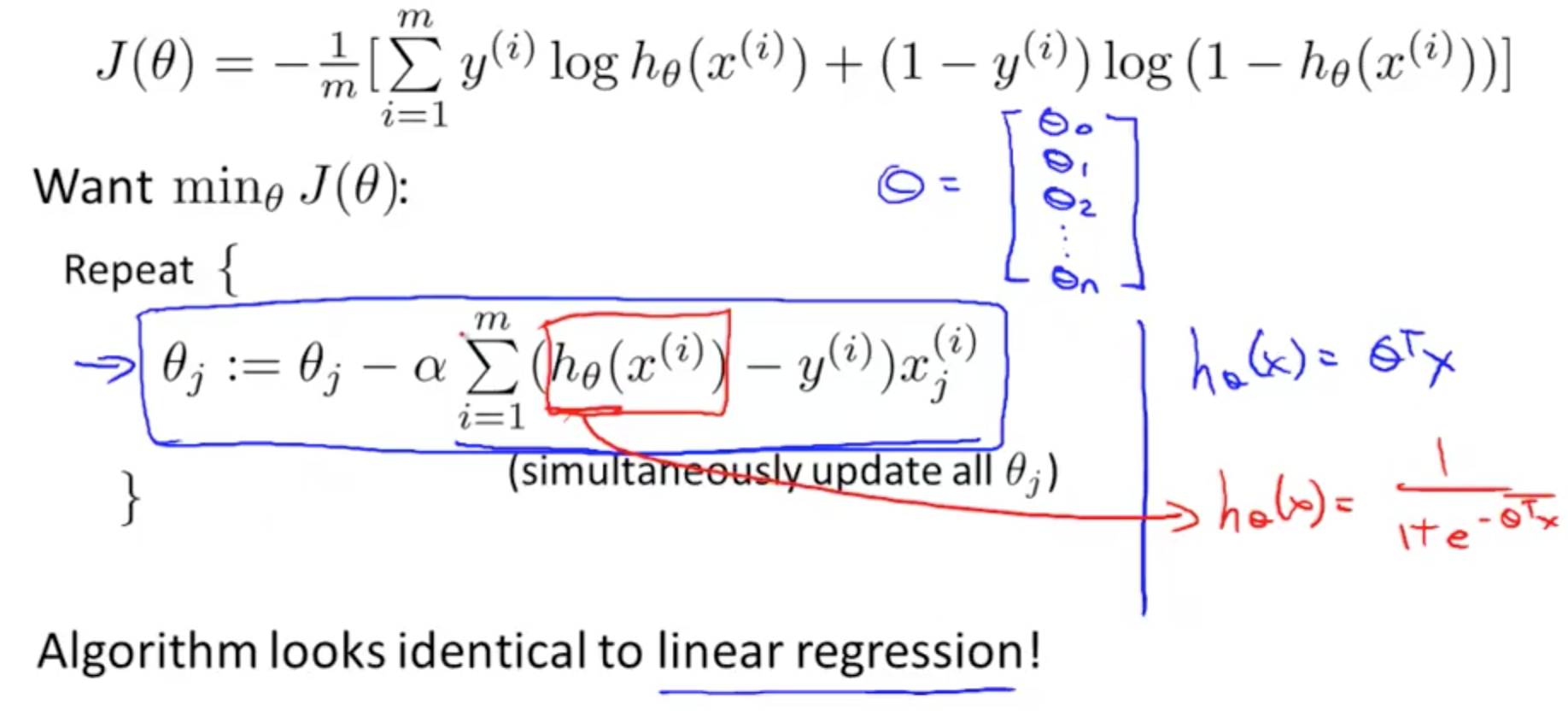
The gradient descent remains the same as discussed in Linear Regression section, the only difference is that now H has changed and so have the cost function. We still have the same formulas, same aim to find a theta such that J is minimized. We again start with some initial theta, update it simultaneously until J is minimized.