Implementing Linear Regression in python

Too much of talks, show me the code.

You can get the code for all the algorithms here: https://github.com/geekRishabhjain/MLpersonalLibrary/tree/master/RlearnPy

The Gradient Descent:

def gradientDescent(self, X, y, alpha, num_iters, theta):
m = y.shape[0]
J_history = np.zeros(shape=(num_iters, 1))
for i in range(num_iters):
predictions = X.dot(theta)  #
theta = theta - (alpha / m) * (((predictions - y).T @ X).T) 
J_history[i] = self.computeCost(X, y, theta)
return [theta, J_history]

Recall what gradient descent was. 'theta' is a matrix of all the thetas, num_iters is the number of times you want to perform the gradient descent. The 'alpha' is the learning rate. X is the matrix of features, and y is a vector for labels.



Each time through the loop, we calculate the predictions for the current theta, this is done by doing the matrix multiplication of X and theta. This gives us a prediction vector of shape same as y.

Note that before feeding X to the function an extra column, for one, the bias term, as discussed earlier had been added to it. This allows theta0 to be updated just like other thetas.

Now we subtract y from h, taking its transpose and multiplying it with x and again taking transpose completes the part inside the summation in gradient descent formula. Finally, we multiply it with alpha over m and subtract it from current theta to generate our new theta.


Each time through the loop, we calculate the cost for the particular choice of theta using the computeCost function, this is stored in J_history. The J_history can be used to ensure that the cost is decreasing with each iteration in the gradient descent.

Implementing the cost function in  python:

def computeCost(self, X, y, theta):
m = X.shape[0]
J = 0
predictions = X.dot(theta)
sqrErrors = np.power(predictions - y, 2)
J = 1 / (2 * m) * np.sum(sqrErrors)
return J

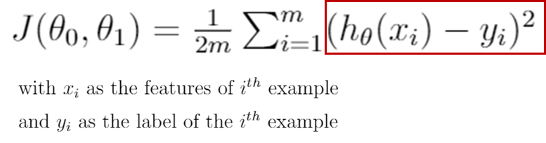
Recall what the cost function for Linear Regression is:

Understanding the code:

First, the predictions are evaluated by doing the matrix multiplication of X and theta. Next, we square the predictions matrix element-wise, np.power function in python lets us do that. To perform the summation in the formula, we use the np.sum function in the numpy library. Finally, we multiply this with one over 2m to get the cost in the variable J.






Note: Before using these functions, add a bias term column in the X. You can do this by using the numpy.append and numpy.ones commands in python. Further, the dimensions of theta should also be appropriately set according to the number of features and the bias term.