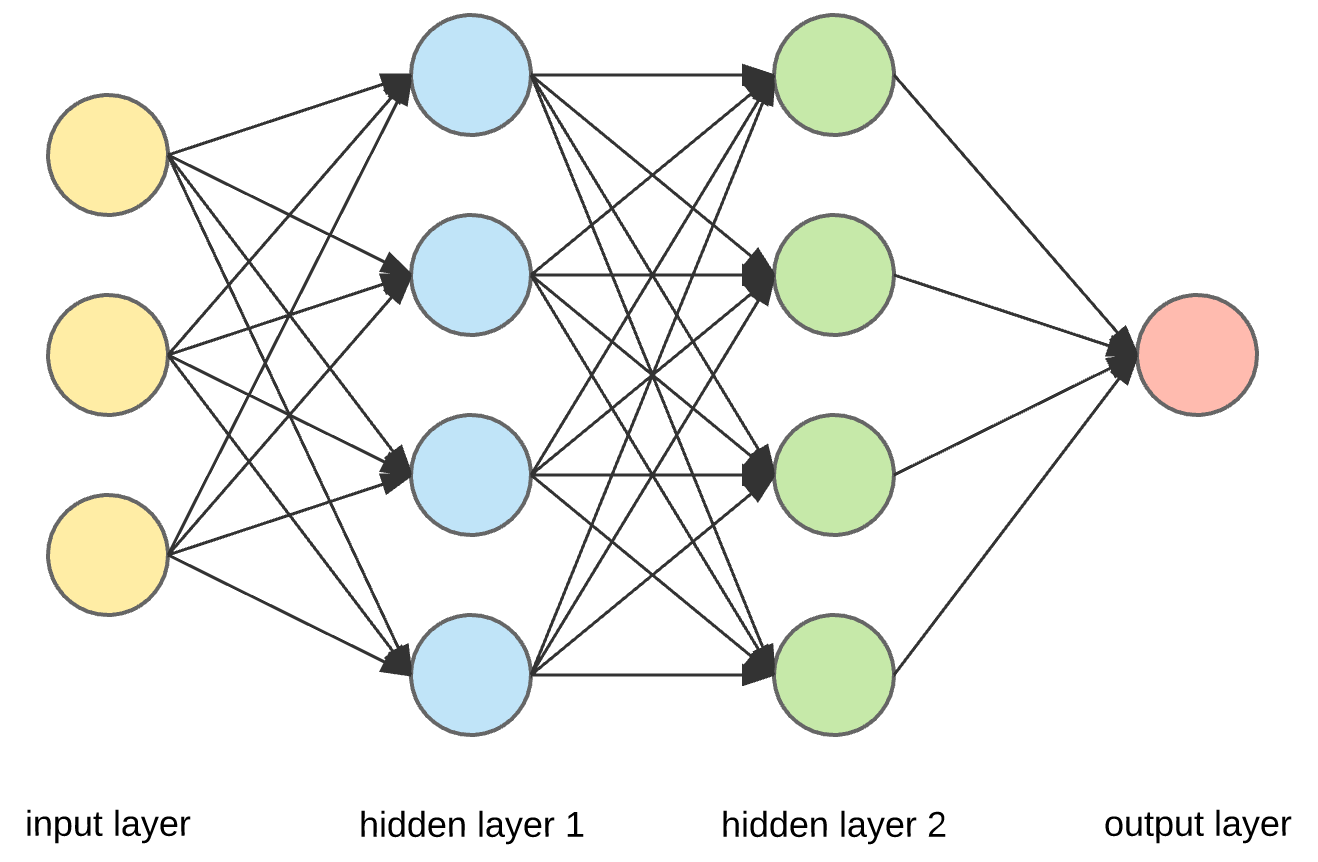
Forward Propagation:

Recall that \[ a(2)(1) = g(theta1(1)(0)*x0 + theta1(1)(1)*x1 + theta1(1)(2)* x2)\],
\[a(2)(2) = g(theta1(2)(0)x0 + theta1(2)(1)x1 + theta1(2)(2)x2)\],
\[a(2)(3) = g(theta1(3)(0)x0 + theta1(3)(1)x1 + theta1(3)(2)x2)\], so on and so forth.
We can vectorize the complete mathematics that neural network does, and it will look better than, then it seems now.
if theta1 is a matrix of dimensions 4*3, and x is a vector of size (3, 1), the activation of each unit in the second layer can be evaluated as follows:
\[a2 = g(theta1@x)\].
Note that we are not counting bias term here, if you want you can add it, you'll only need to add one to each activation vector at each step and @ is the operator for matrix multiplication in python.
Now, similarly the activations in the third layer can be evaluated as follows:
\[a3 = g(theta2@a2)\]
And finally the output can be calculated as:
\[h(x) = g(theta3@a3)\].
This was all about predicting, given thetas how to predict the output for a set of features. In an upcoming post, we'll learn how to train Neural Network to learn the thetas.
No comments:
Post a Comment